Post-Training for Large Language Models: Theory and Practice

1. Overview

Post-training is the stage that follows large-scale pretraining of language models. While pretraining teaches a model to predict the next token from massive text corpora, post-training adapts it to follow instructions, align with human intent, and behave safely. Key methods include Supervised Fine-Tuning (SFT), Reinforcement Learning from Human Feedback (RLHF), and newer Direct Preference Optimization (DPO) techniques. The goal is no longer to mimic raw text but to optimize for human-defined qualities such as helpfulness, harmlessness, and honesty.

Modern systems like OpenAI's InstructGPT [1], Anthropic's Claude [2], and Meta's Llama-3-Chat [3] all rely on these post-training steps.

This document explores the reinforcement learning techniques underlying modern LLM post-training, integrating theoretical foundations with practical implementation experience. We begin with classical RL fundamentals and policy gradient methods, then examine how preference learning adapts these techniques for language models, and finally explore modern approaches like reward modeling with PPO and Direct Preference Optimization (DPO).

2. Reinforcement Learning Fundamentals

Reinforcement learning (RL) is a framework where an agent learns to make decisions by interacting with an environment, receiving rewards or penalties based on its actions, and optimizing its policy to maximize cumulative rewards.

2.1 RL Setup and Notation

The standard RL problem is formalized as a Markov Decision Process (MDP) defined by the tuple $(\mathcal{S}, \mathcal{A}, \mathcal{P}, \mathcal{R}, \gamma)$:

• States $s \in \mathcal{S}$: Observations of the environment
• Actions $a \in \mathcal{A}$: Choices the agent can make
• Transition dynamics $\mathcal{P}(s'|s, a)$: Probability of transitioning to state $s'$ given state $s$ and action $a$
• Reward function $\mathcal{R}(s, a)$: Scalar feedback signal
• Discount factor $\gamma \in [0, 1]$: Trade-off between immediate and future rewards
• Policy $\pi_\theta(a|s)$: The agent's strategy, parameterized by $\theta$
• Trajectory $\tau = (s_0, a_0, s_1, a_1, \ldots, s_T, a_T)$: A sequence of states and actions
• Return $R(\tau) = \sum_{t=0}^{T} \gamma^t r_t$: Cumulative discounted reward

The goal of RL is to find the optimal policy $\pi^*$ that maximizes the expected return:

Two popular classes of algorithms for solving this optimization problem are on-policy and off-policy methods.

2.2 On-Policy vs Off-Policy Methods

On-policy methods learn from data generated by the current policy being optimized. The agent collects experience by following its current policy $\pi_\theta$, uses that data to update the policy, and then discards it. This ensures the training data distribution always matches the policy's behavior, but requires fresh data collection after each update. Examples include REINFORCE, A2C, and PPO.

Off-policy methods can learn from data generated by different policies (including older versions or human demonstrations). The agent maintains a replay buffer and can reuse data multiple times. This improves sample efficiency but introduces distribution mismatch challenges. Examples include Q-learning, DQN, and SAC.

Why On-Policy for RLHF?

For LLM fine-tuning, on-policy methods (like PPO) are strongly preferred for several reasons:

1. Distribution Shift Problem. Language models operate in an enormous state-action space (vocabulary size of 50k+, sequence lengths of 1000+). As the policy improves, the distribution of generated text changes dramatically. Off-policy methods struggle when this mismatch compounds in high-dimensional spaces.

2. Importance Sampling Challenges. Off-policy methods rely on importance weights $\frac{\pi_\theta(a|s)}{\pi_\text{old}(a|s)}$, which become extremely large or small in language generation, making learning unstable.

3. Reward Model Generalization. The reward model is trained on a fixed distribution. On-policy methods with KL penalties keep the policy closer to the reference distribution where the reward model is trustworthy.

4. Sample Efficiency Trade-off. Generating text is relatively cheap compared to training the model. The stability of on-policy methods outweighs any sample efficiency gains from reusing old trajectories.

2.3 Evolution of Policy Gradient Methods

Having established why on-policy methods are preferred for RLHF, we now trace the evolution of policy gradient algorithms. Each builds on its predecessors' insights while introducing innovations that make training more practical and reliable.

2.4 REINFORCE

REINFORCE is a foundational policy gradient algorithm that directly optimizes the policy by following the gradient of expected rewards. The policy gradient theorem gives us:

where $\theta$ are the policy parameters, $\tau$ is a trajectory, $R(\tau)$ is the return, and $\pi_\theta(a_t | s_t)$ is the probability of taking action $a_t$ in state $s_t$.

While conceptually simple and unbiased, REINFORCE suffers from high variance in gradient estimates, which makes training unstable and sample-inefficient.

2.5 REINFORCE with Baseline

A simple but powerful improvement is subtracting a baseline from the returns, which doesn't introduce bias but dramatically reduces variance. The most common baseline is the value function $V(s_t)$:

2.6 Actor-Critic Methods

Actor-critic methods combine policy optimization with value function learning. The "actor" is the policy network; the "critic" is a value function that estimates expected future rewards. The gradient update uses the advantage function:

where $A(s_t, a_t) = Q(s_t, a_t) - V(s_t)$ represents how much better an action is compared to the average. The critic provides immediate feedback without waiting for trajectory completion, enabling more frequent updates and faster convergence.

2.7 Trust Region Policy Optimization (TRPO)

TRPO constrains optimization steps to lie within a "trust region" by limiting the KL divergence between old and new policies:

subject to: $\mathbb{E}_{s \sim \pi_{\theta_\text{old}}} [D_\text{KL}(\pi_{\theta_\text{old}}(\cdot|s) \| \pi_\theta(\cdot|s))] \leq \delta$

While TRPO provides strong theoretical guarantees and stable training, its second-order optimization procedure is computationally expensive and difficult to scale to large models.

2.8 Proximal Policy Optimization (PPO)

PPO simplifies TRPO while retaining most of its benefits. Instead of explicitly constraining KL divergence, PPO uses a clipped surrogate objective:

where $r_t(\theta) = \frac{\pi_\theta(a_t|s_t)}{\pi_{\theta_\text{old}}(a_t|s_t)}$ is the probability ratio and $\epsilon$ (typically 0.2) controls the clipping range. This requires only first-order gradients yet provides stable training with monotonic improvement.

2.9 Experimental Results: On-Policy Methods on CartPole

The figure below compares the four on-policy algorithms, each evaluated over 1,000 episodes and averaged across 20 independent simulation runs on CartPole-v1.

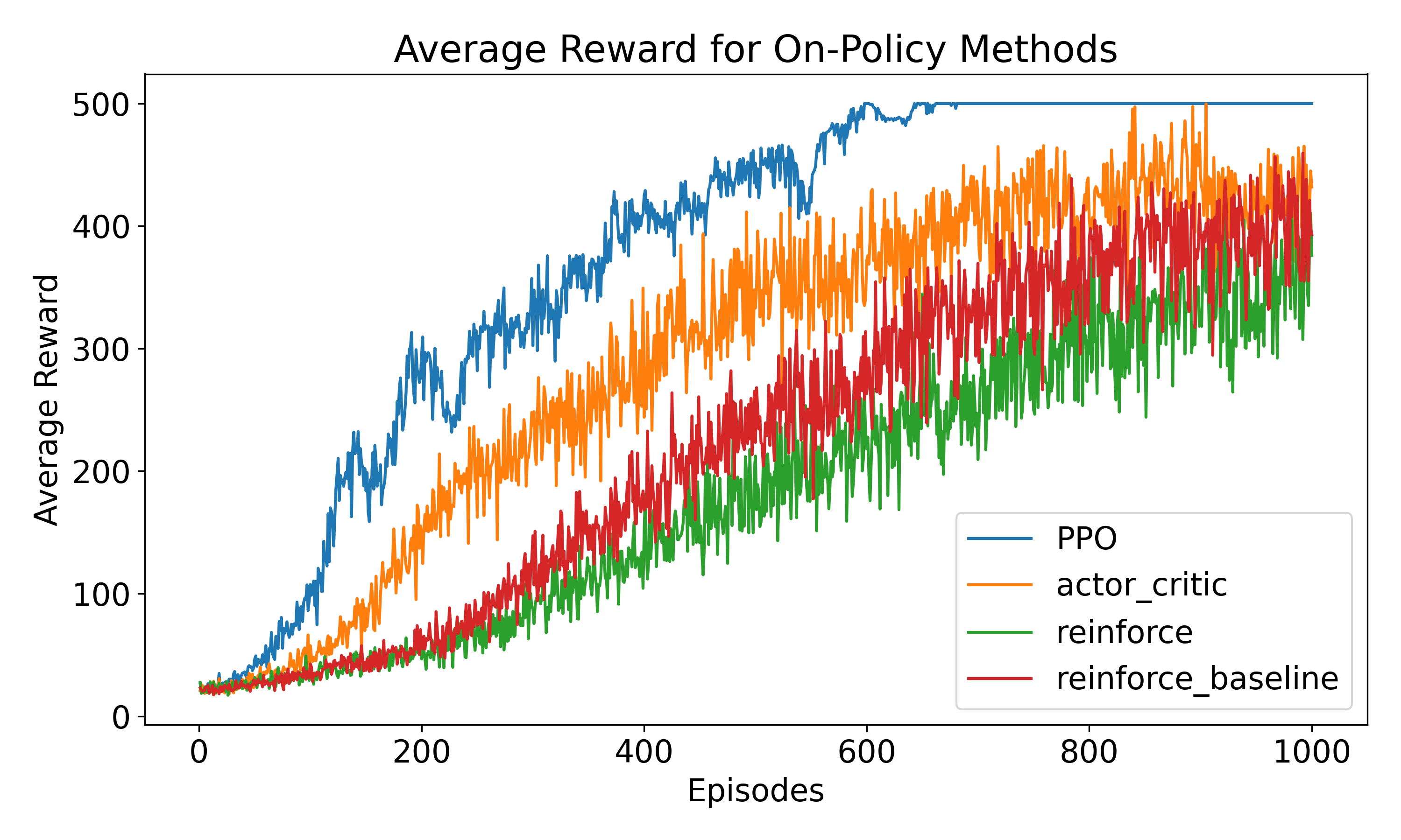
The results highlight the progression in algorithmic maturity. Vanilla REINFORCE converges slowest with the highest variance—a direct consequence of full Monte Carlo returns without variance reduction. Adding a learned baseline substantially stabilizes learning and accelerates convergence. Actor-Critic pushes further by bootstrapping value estimates at every timestep. PPO achieves the best final performance and most consistent convergence; the clipped surrogate objective prevents destructive large updates, which is why it has become the default on-policy algorithm for RLHF.

3. Preference Learning for LLMs

Preference learning differs fundamentally from classical RL by learning from comparative judgments rather than absolute reward signals. Instead of providing scalar rewards, humans compare two or more model outputs and indicate which is preferred. This approach is particularly suitable for LLM fine-tuning because defining an explicit reward function for open-ended text generation is extremely difficult—concepts like "helpfulness" and "honesty" are complex and context-dependent.

Preference learning aligns naturally with how humans evaluate language: we can more reliably say "response A is better than response B" than assign absolute numerical scores. This comparative approach reduces labeling inconsistencies and captures subtle trade-offs between quality dimensions.

4. Reward Modeling with PPO

The reward modeling + PPO approach, popularized by InstructGPT [1], decomposes RLHF into two phases. First, a reward model is trained on human preference data using a ranking loss:

where $x$ is the prompt, $y_w$ is the preferred response, $y_l$ is the rejected response, and $r_\phi$ is the reward model. Once trained, PPO fine-tunes the language model using this reward signal:

The KL penalty prevents the model from drifting too far from the reference policy $\pi_\text{ref}$—without it, the model might exploit weaknesses in the reward model or generate nonsensical text that happens to score well.

This two-stage approach is powerful but has notable challenges. The reward model can be a bottleneck, as prediction errors compound during RL training. The optimization is computationally expensive, requiring multiple rollouts, reward evaluations, and value function updates. Additionally, the reward model may not generalize to the distribution produced by the increasingly optimized policy, leading to reward hacking.

5. Direct Preference Optimization (DPO)

DPO [6] eliminates the need for a separate reward model by deriving a closed-form mapping between the optimal RL policy and the reward function. The DPO loss is:

Given a preference pair, DPO increases the likelihood of the preferred response while decreasing the likelihood of the rejected one, all while maintaining a KL penalty to the reference policy. This is mathematically equivalent to reward modeling + PPO under certain assumptions, but far simpler.

DPO is often preferred over PPO for several reasons: it requires only supervised learning infrastructure (no value networks, advantage estimation, or sampling passes); the supervised objective is more stable and less prone to reward hacking; it eliminates error compounding from a separate reward model; and it has fewer hyperparameters to tune.

6. Learning Roadmap

If you're following a similar path, here is the progression I recommend:

Start with Classical RL (CartPole). Implement vanilla REINFORCE to understand policy gradients. Add a baseline to see variance reduction in action. Progress to actor-critic for value function estimation. Implement PPO to understand trust regions and stable optimization.

Understand the Transition to Preferences. Read Christiano et al. [4] on learning from human preferences. Understand why preferences work better than absolute rewards for language tasks. Study the reward modeling + PPO pipeline.

Hands-on with LLM Fine-tuning. Start with DPO (simpler than reward modeling + PPO). Use HuggingFace's TRL library for infrastructure. Fine-tune a small model (GPT-2) before scaling up.

Dive Deeper. Experiment with different $\beta$ values. Try different datasets (HH-RLHF, summarization). Compare reference model vs. fine-tuned outputs. Read recent papers on improvements (IPO, KTO, etc.).

References

- Ouyang, L., Wu, J., Jiang, X., et al. (2022). Training language models to follow instructions with human feedback. NeurIPS 35, 27730–27744.
- Bai, Y., Kadavath, S., Kundu, S., et al. (2022). Constitutional AI: Harmlessness from AI feedback. arXiv:2212.08073.
- Meta AI. (2024). Llama 3 Model Card.
- Christiano, P. F., Leike, J., Brown, T., et al. (2017). Deep reinforcement learning from human preferences. NeurIPS 30.
- Schulman, J., Wolski, F., Dhariwal, P., et al. (2017). Proximal policy optimization algorithms. arXiv:1707.06347.
- Rafailov, R., Sharma, A., Mitchell, E., et al. (2023). Direct preference optimization: Your language model is secretly a reward model. NeurIPS 36.
- Schulman, J., Levine, S., Abbeel, P., et al. (2015). Trust region policy optimization. ICML, 1889–1897.
- Williams, R. J. (1992). Simple statistical gradient-following algorithms for connectionist reinforcement learning. Machine Learning, 8(3), 229–256.
- Sutton, R. S. & Barto, A. G. (2018). Reinforcement Learning: An Introduction (2nd ed.). MIT Press.